Introduction

What is the Megabot?

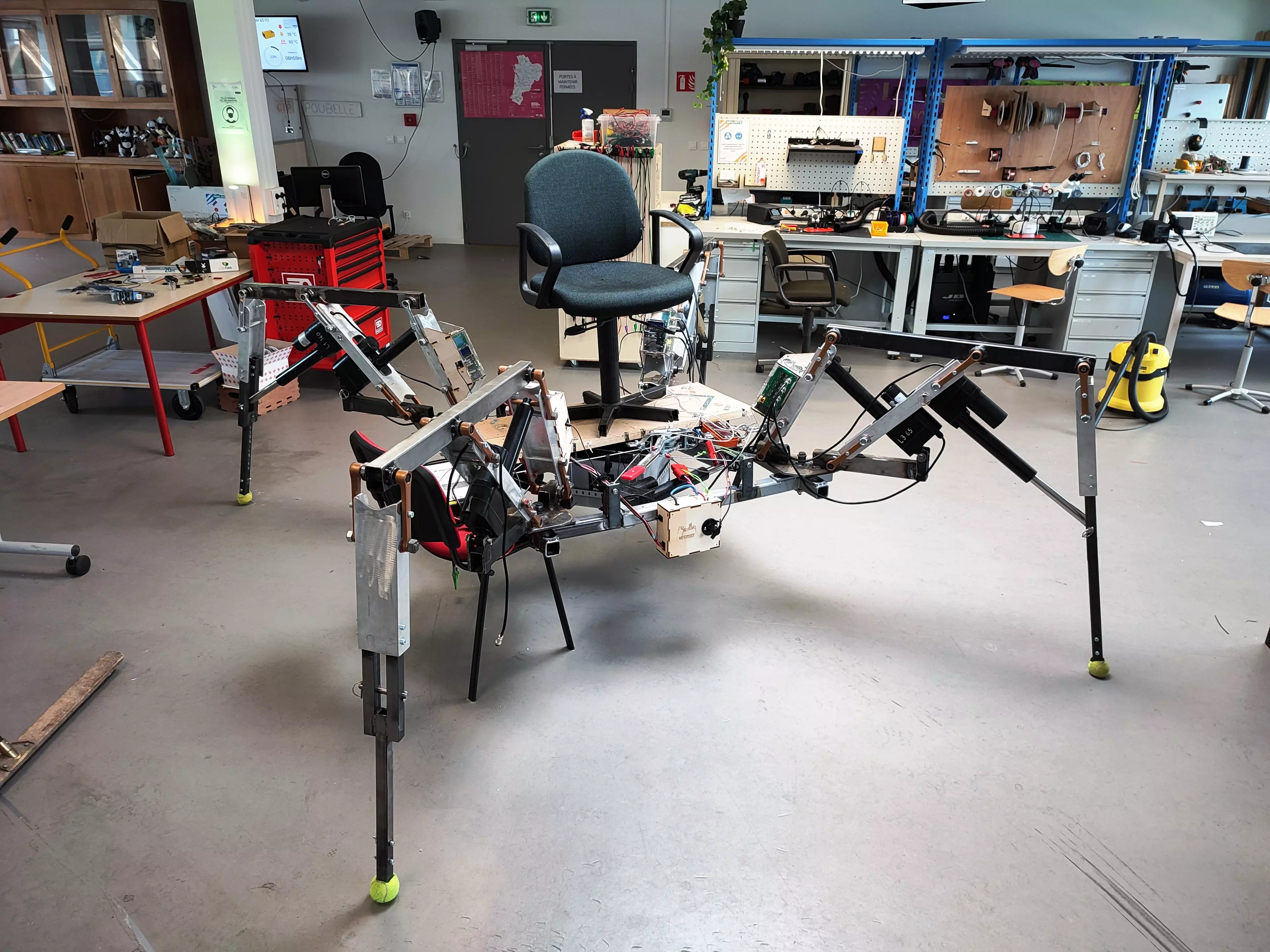
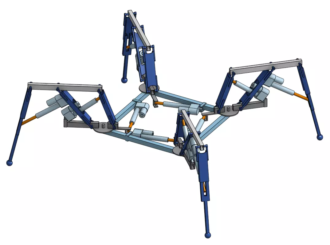
The Megabot is a large quadrupedal robot capable of carrying a passenger, primarily designed to be showcased at robotics-related events. It weighs approximately 250 kg, measures around 2.50 m in width, and operates via electric actuators. Its design and construction were carried out by Julien Allali , a lecturer at ENSEIRB-MATMECA, and it is currently housed at the Fablab of Bordeaux INP.

Mission

The primary goal of this project is to refine the robot’s control by improving its kinematic model, meaning revising all algorithms that translate a position command into an actuator elongation command. After that, the aim is to implement a walking algorithm so that the robot can follow a curved trajectory. Finally, to validate the implemented algorithms independently of real-world constraints such as structural deformation due to weight, the Megabot must be modeled and integrated into the PyBullet simulator.  

Control

The goal of control is to establish the inverse kinematics of the Megabot, meaning implementing a set of methods to determine the elongations of the 12 actuators needed to achieve a given position. In general, inverse kinematics can be computed using dedicated libraries by providing them with a URDF model of the robot (for example, Pinocchio in Python). However, this approach could not be implemented for the Megabot for two reasons:

• The URDF format constructs a tree where the nodes represent the robot’s parts and the edges represent the joints between them (slider, pivot, etc.). Since the Megabot’s structure includes geometric loops, this would introduce cycles in the tree, which is not allowed.

• If we were to model the Megabot as a tree by removing its geometric loops and simulating a robot actuated by motors at its joints, we would then be minimizing the error in our inverse kinematics based on joint angles rather than actuator elongations.

We have therefore decided to clearly redefine the Megabot’s kinematics.

Megabot Kinematics

Establishing the forward kinematic model of a robot means developing a set of computational methods to determine the robot’s position based on given joint values. In our case, this involves creating one or more functions that take valid actuator elongations as input and return the Megabot’s position. This problem can be solved analytically quite easily.

Establishing the inverse kinematic model, however, is the reverse process: we want to determine joint values from a given position. This is significantly more complex than forward kinematics and often cannot be solved analytically, including in the case of the Megabot.

A common approach to solving this problem is to use the Jacobian matrix associated with the forward kinematic model. This matrix consists of the partial derivatives of the forward kinematics and allows for a linear approximation of the relationship between joint values and position values for small variations. Once this Jacobian \(J\) is determined, the inverse kinematics problem can be solved by formulating a quadratic optimization problem:

In this problem, \(\Delta V\) is the vector of actuator elongation variations to be determined, \(J\) is the Jacobian of the forward kinematics, and \(\Delta X\) is the vector of position variations. The goal is to minimize the quadratic error on \(\Delta X\) while constraining \(\Delta V\) with variables \(G\), \(h\), \(A\), \(b\), \(lb\), and \(ub\). These constraint variables are useful for ensuring actuator elongations remain within their physical limits.

Demonstration Details

This approach to solving inverse kinematics is an example of applying the least squares method. Solving this quadratic problem can be done using a QP solver such as \(\verb|qpsolvers|\) in Python.

Calculation of the Jacobian for Direct Kinematics

We will now develop the Jacobian matrix associated with the direct kinematics of the Megabot. We will first construct it relative to a single leg in its plane before generalizing it to all legs in the world reference frame.

Direct Kinematics in the Leg Plane

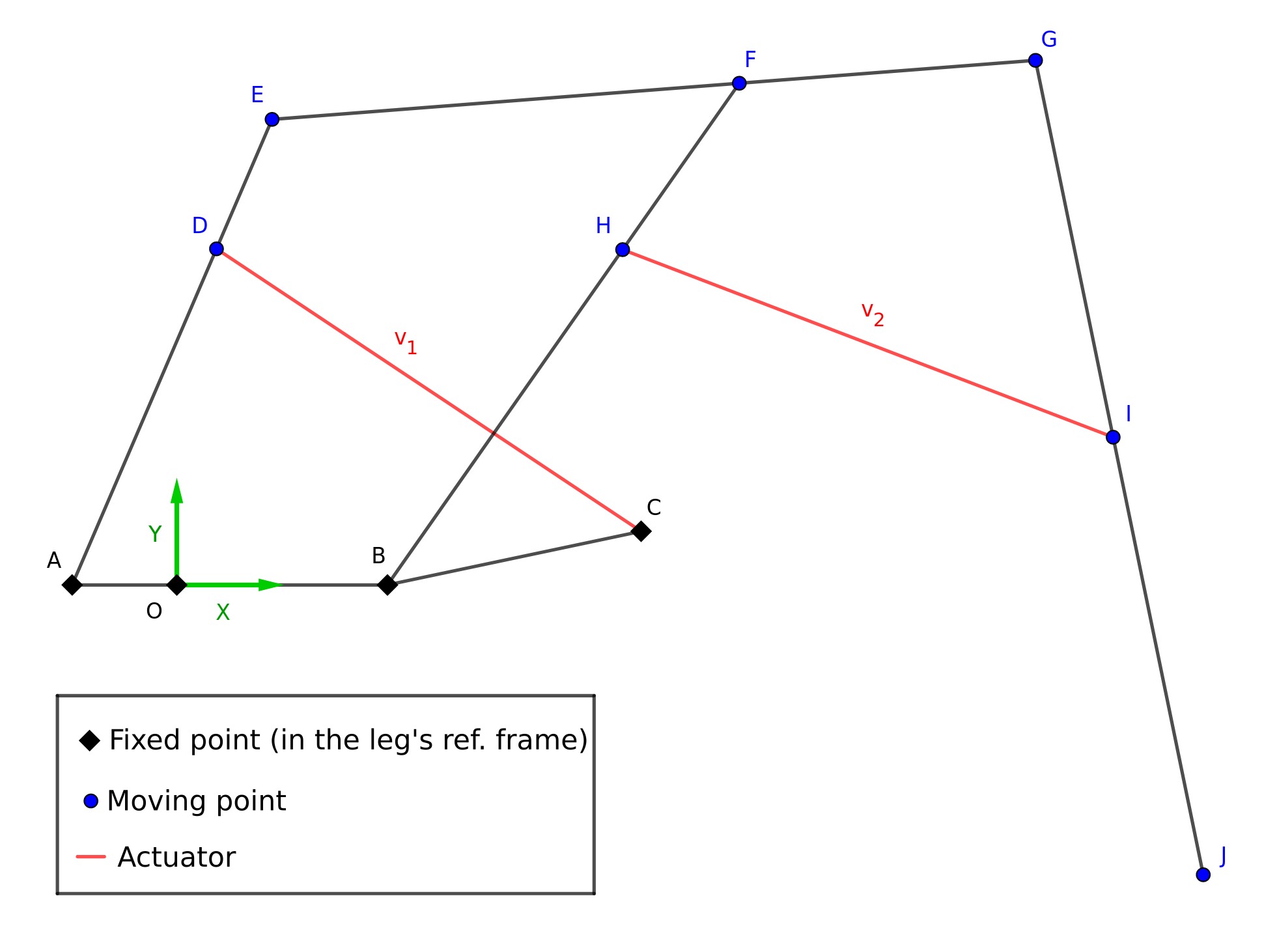
To determine the Jacobian associated with our direct kinematics in the leg plane, it is necessary to formalize our problem. We will successively compute the position deviations of points \(D\), \(E\), \(F\), \(G\), \(H\), \(I\) and \(J\), represented in the following diagram, as a function of the elongation variations \(\Delta v_1\) and \(\Delta v_2\) of the actuators.

These calculations result in obtaining the matrix \(M_J\) such that:

We then notice that this matrix is the Jacobian \(J_2\) associated with our direct kinematic model in the leg plane:

Details of the Deviation Calculations

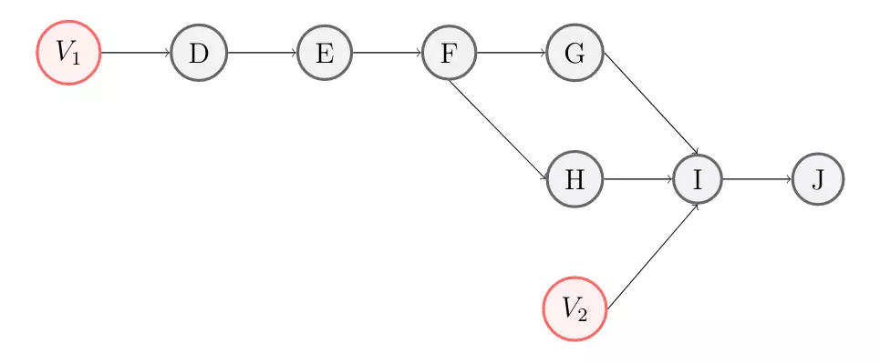
For 2 points \(A\) and \(B\) separated by a constant distance, we denote their separation as \(d_{AB}\). The dependency graph of the leg’s joints is as follows:

 

First, we seek to determine the deviation at \(D\). For this, we consider the triangle \(ADC\), where the elongation \(v_1\) of segment \(CD\) and the position of point \(D\) are variable. We obtain the following system \(S_{1}\):

\begin{equation*} S_{1} \left \{ \begin{array}{l} \left\langle \overrightarrow{AD} \middle| \overrightarrow{AD} \right\rangle - d_{AD}^{\hspace{0.1cm}2} = (x_{D} - x_{A})^{2} + (y_{D} - y_{A})^{2} - d_{AD}^{\hspace{0.1cm}2} = 0 \\ ~\\ \left\langle \overrightarrow{CD} \middle| \overrightarrow{CD} \right\rangle - v_{1}^{\hspace{0.1cm} 2} = (x_{D} - x_{C})^{2} + (y_{D} - y_{C})^{2} - v_{1}^{\hspace{0.1cm} 2} = 0 \\ \end{array} \right. \end{equation*}

 

After differentiation with respect to \(x_{D}\), \(y_{D}\) and \(v_1\), and assuming that \(A\), \(D\) and \(C\) are not collinear (which is always verified due to the leg structure), system \(S_{1}\) gives us the following matrix relation:

\begin{equation*} \nabla S_{1_{D, v_1}} \cdot \begin{bmatrix} \Delta x_{D}\\ \Delta y_{D}\\ \Delta v_1\\ \end{bmatrix} = \begin{bmatrix} 2(x_{D} - x_{A}) & 2(y_{D} - y_{A}) & 0 \\ 2(x_{D} - x_{C}) & 2(y_{D} - y_{C}) & -2v_{1} \end{bmatrix} \cdot \begin{bmatrix}\Delta x_{D}\\ \Delta y_{D}\\ \Delta v_1\\ \end{bmatrix} = \begin{bmatrix}0\\0\end{bmatrix} \end{equation*}

 

\begin{equation*} \Longrightarrow \hspace{0.5cm} \Delta D = \begin{bmatrix}\Delta x_{D}\\ \Delta y_{D} \end{bmatrix} = \begin{bmatrix} 2(x_{D} - x_{A}) & 2(y_{D} - y_{A}) \\ 2(x_{D} - x_{C}) & 2(y_{D} - y_{C}) \end{bmatrix}^{-1} \cdot \begin{bmatrix} 0 \\ 2v_{1} \end{bmatrix} \cdot \Delta v_{1} \end{equation*}

 

\begin{equation*} \boxed{ \Delta D = M_D \cdot \Delta v_{1} \hspace{0.2cm} \text{with} \hspace{0.2cm} M_D = \begin{bmatrix} 2(x_{D} - x_{A}) & 2(y_{D} - y_{A}) \\ 2(x_{D} - x_{C}) & 2(y_{D} - y_{C}) \end{bmatrix}^{-1} \cdot \begin{bmatrix} 0 \\ 2v_{1} \end{bmatrix} } \end{equation*}

 

Since the points \(A\), \(D\) and \(E\) are collinear, the position deviation at \(E\) can be determined from the deviation at \(D\) by applying a simple proportionality factor.

\begin{equation*} \boxed{\Delta E = M_E \cdot \Delta v_1 \hspace{0.2cm} \text{with} \hspace{0.2cm} M_E = \dfrac{d_{AE}}{d_{AD}} \cdot M_D } \end{equation*}

 

We now calculate the displacement at \(F\) by considering the triangle \(EBF\), where the positions of points \(E\) and \(F\) are variable. We obtain the following system \(S_2\):

\begin{equation*} S_{2} \left \{ \begin{array}{l} \left\langle \overrightarrow{EF} \middle| \overrightarrow{EF} \right\rangle - d_{EF}^{\hspace{0.1cm}2} = (x_{F} - x_{E})^{2} + (y_{F} - y_{E})^{2} - d_{EF}^{\hspace{0.1cm}2} = 0 \\ ~\\ \left\langle \overrightarrow{BF} \middle| \overrightarrow{BF} \right\rangle - d_{BF}^{\hspace{0.1cm}2} = (x_{F} - x_{B})^{2} + (y_{F} - y_{B})^{2} - d_{BF}^{\hspace{0.1cm}2} = 0 \\ \end{array} \right. \end{equation*}

 

We differentiate it with respect to \(x_{F}\), \(y_{F}\), \(x_{E}\) and \(y_{E}\), and under the condition that \(B\), \(E\) and \(F\) are not collinear (which is always verified due to the leg’s structure), we obtain:

\begin{equation*} \nabla S_{2_{F, E}} \cdot \begin{bmatrix} \Delta x_{F} \\ \Delta y_{F} \\ \Delta x_{E} \\ \Delta y_{E} \end{bmatrix} = \begin{bmatrix} 2(x_{F} - x_{E}) & 2(y_{F} - y_{E}) & -2(x_{F} - x_{E}) & -2(y_{F} - y_{E}) \\ 2(x_{F} - x_{B}) & 2(y_{F} - y_{B}) & 0 & 0 \end{bmatrix} \cdot \begin{bmatrix} \Delta x_{F} \\ \Delta y_{F} \\ \Delta x_{E} \\ \Delta y_{E} \end{bmatrix} = \begin{bmatrix} 0\\ 0\\ 0\\ 0\\ \end{bmatrix} \end{equation*}

 

\begin{equation*} \Longrightarrow \hspace{0.5cm} \Delta F = \begin{bmatrix} \Delta x_{F}\\ \Delta y_{F} \end{bmatrix} = \begin{bmatrix} 2(x_{F} - x_{E}) & 2(y_{F} - y_{E}) \\ 2(x_{F} - x_{B}) & 2(y_{F} - y_{B}) \\ \end{bmatrix}^{-1} \cdot \begin{bmatrix} 2(x_{F} - x_{E}) & 2(y_{F} - y_{E}) \\ 0 & 0 \end{bmatrix} \cdot \Delta E \end{equation*}

 

\begin{equation*} \boxed{\Delta F = M_F \cdot \Delta v_1 \hspace{0.2cm} \text{with} \hspace{0.2cm} M_F = \begin{bmatrix} 2(x_{F} - x_{E}) & 2(y_{F} - y_{E}) \\ 2(x_{F} - x_{B}) & 2(y_{F} - y_{B}) \\ \end{bmatrix}^{-1} \cdot \begin{bmatrix} 2(x_{F} - x_{E}) & 2(y_{F} - y_{E}) \\ 0 & 0 \end{bmatrix} \cdot M_E} \end{equation*}

 

The points \(E\), \(F\) and \(G\) on one hand, and \(B\), \(F\) and \(H\) on the other hand, are collinear. Therefore, the position changes in \(G\) and \(H\) can be derived from the change in \(F\) :

\begin{equation*} \boxed{\Delta G = M_{G} \cdot \Delta v_{1} \hspace{0.2cm} \text{with} \hspace{0.2cm} M_G = \dfrac{d_{EG}}{d_{EF}} \cdot M_F} \end{equation*}

 

\begin{equation*} \boxed{\Delta H = M_{H} \cdot \Delta v_{1} \hspace{0.2cm} \text{with} \hspace{0.2cm} M_H = \dfrac{d_{BH}}{d_{BF}} \cdot M_F} \end{equation*}

 

We can now calculate the deviation at \(I\) by considering the triangle \(GHI\), where the positions of points \(G\) and \(H\), as well aw the elongation \(v_2\) of the segment \(HI\), are variable. We obtain the following system \(S_3\):

\begin{equation*} S_{3} \left \{ \begin{array}{l} \left\langle \overrightarrow{GI} \middle| \overrightarrow{GI} \right\rangle - d_{GI}^{\hspace{0.1cm}2} = (x_{I} - x_{G})^{2} + (y_{I} - y_{G})^{2} - d_{GI}^{\hspace{0.1cm}2} = 0 \\ ~\\ \left\langle \overrightarrow{HI} \middle| \overrightarrow{HI} \right\rangle - v_{2}^{\hspace{0.1cm} 2} = (x_{I} - x_{H})^{2} + (y_{I} - y_{H})^{2} - v_{2}^{\hspace{0.1cm} 2} = 0 \\ \end{array} \right. \end{equation*}

 

We differentiate it with respect to \(x_{I}\), \(y_{I}\), \(x_{G}\), \(y_{G}\), \(x_{H}\), \(y_{H}\) and \(v_{2}\) to obtain the following Jacobian:

\begin{equation*} \nabla S_{3_{I, G, H, v_{2}}} = \begin{bmatrix} M_{1} & -M_{2} & -M_{3} & -M_{4} \end{bmatrix} \hspace{0.2cm} \text{with} \end{equation*}

 

\begin{equation*} M_1 = \begin{bmatrix} 2(x_{I} - x_{G}) & 2(y_{I} - y_{G}) \\ 2(x_{I} - x_{H}) & 2(y_{I} - y_{H}) \end{bmatrix} \hspace{2cm} M_2 = \begin{bmatrix} 2(x_{I} - x_{G}) & 2(y_{I} - y_{G}) \\ 0 & 0 \end{bmatrix} \end{equation*}

 

\begin{equation*} \hspace{-3.55cm} M_3 = \begin{bmatrix} 0 & 0 \\ 2(x_{I} - x_{H}) & 2(y_{I} - y_{H}) \end{bmatrix} \hspace{2cm} M_4 = \begin{bmatrix} 0 \\ 2 v_2 \end{bmatrix} \end{equation*}

 

We then have the following relation that links the displacement at \(I\) to \(\Delta v_1\) and \(\Delta v_2\), under the condition that \(I\), \(G\) and \(H\) are not aligned (which is always verified due to the structure of the leg):

\begin{equation*} \Delta I = M_{1}^{-1} \cdot \left( M_{2} \cdot \Delta G + M_{3} \cdot \Delta H + M_{4} \cdot \Delta v_{2} \right) = M_{1}^{-1} \cdot \left( M_{2} \cdot M_{G} + M_{3} \cdot M_{H} \right) \cdot \Delta v1 + M_{1}^{-1} \cdot M_{4} \cdot \Delta v_{2} \end{equation*}

 

\begin{equation*} \boxed{ \array{ \Delta I = M_I \cdot \begin{bmatrix} \Delta v_{1}\\ \Delta v_{2} \end{bmatrix} \\[0.2cm] \text{with} \\[0.2cm] \hspace{0.2cm} M_I = \begin{bmatrix} V1 & V2 \end{bmatrix} \hspace{1cm} V_1 = M_{1}^{-1} \cdot \left( M_{2} \cdot M_{G} + M_{3} \cdot M_{H} \right) \hspace{1cm} V_2 = M_{1}^{-1} \cdot M_{4} \hspace{0.2cm}}} \end{equation*}

 

Finally, because \(G\), \(I\) and \(J\) are aligned, we obtain the displacement at \(J\):

\begin{equation*} \boxed{\Delta J = M_J \cdot \begin{bmatrix} \Delta v_{1}\\ \Delta v_{2} \end{bmatrix} \hspace{0.2cm} \text{with} \hspace{0.2cm} M_J = \dfrac{d_{GJ}}{d_{GI}} \cdot M_I} \end{equation*}

 

Direct Kinematics in the Leg’s Space

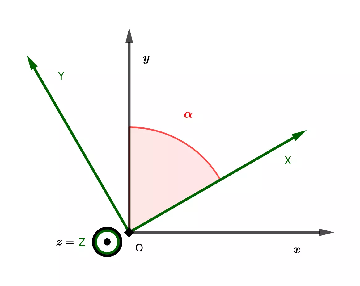
The goal now is to bring our model into space by adding the influence of the actuator \(v_3\) to our direct kinematics. The target reference frame is the frame \((\overrightarrow{x}, \overrightarrow{y}, \overrightarrow{z})\), represented in the following figure. It is worth noting that the vector \(\overrightarrow{Y}\), used in the previous part, has become the vector \(\overrightarrow{Z}\) in this modeling for the sake of convention.

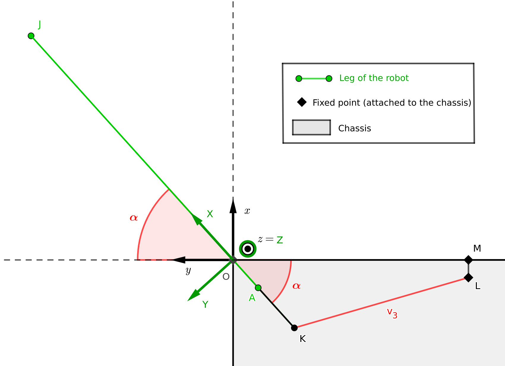
Let \((X, Z)\) be the coordinates of the foot’s tip \(J\) in its plane. First, we need to express the angle \(\alpha\) of the leg relative to the chassis as a function of the elongation of the actuator \(v_3\). This will allow us to derive expressions for the variations of \(X\), \(Z\) and \(\alpha\) as functions of the variations \(v_1\), \(v_2\) and \(v_3\).

Once this relationship is explicit, we need to translate the rotation by an angle \(\alpha\) around the axis \(\overrightarrow Z\) into a matrix form in order to transform into the reference frame \((\overrightarrow x, \overrightarrow y, \overrightarrow z)\). We then obtain the following relationship:

From the matrices \(A\) and \(B\), it becomes possible to construct \(J_3\), the matrix that relates \((\Delta x, \Delta y, \Delta z)\) to \((\Delta v_1, \Delta v_2, \Delta v_3)\):

Details of the coordinate frame change

First, we aim to express the angle \(\alpha\) First, we aim to express the angle \(v_3\). To do this, we place ourselves in the triangle \(KLO\).

 

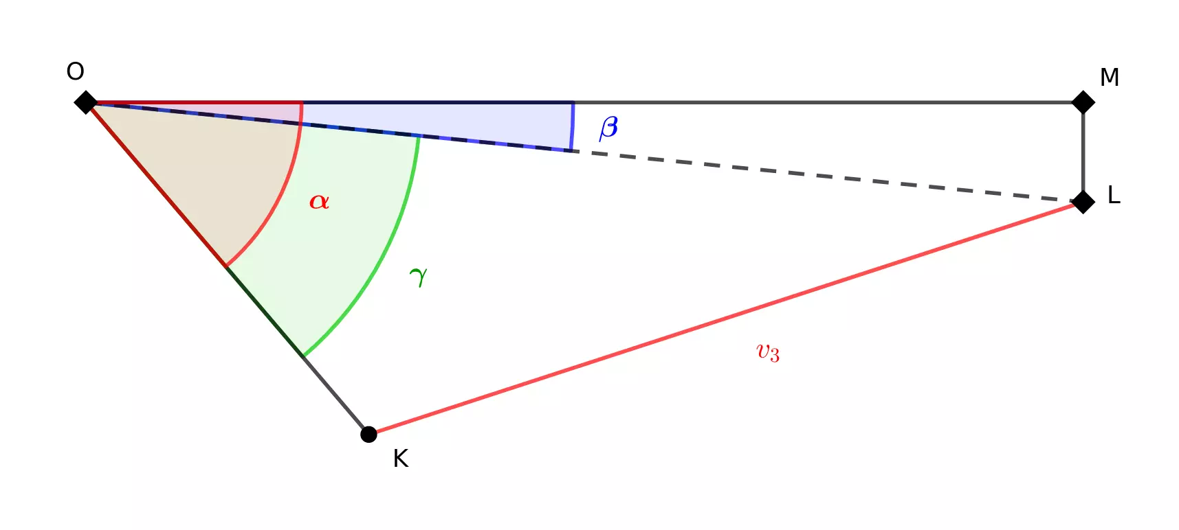
Using the law of cosines, we obtain the following relation:

\begin{equation*} \begin{array}{lc} &d_{OK} \cdot d_{OL} \cdot \cos{\gamma} = \dfrac{1}{2} ( d_{OK}^{\hspace{0.1cm} 2} + d_{OL}^{\hspace{0.1cm} 2} - v_3^{\hspace{0.1cm} 2}) \\~\\ \implies & \dfrac{d_{OK}}{d_{OL}} + \dfrac{d_{OL}}{d_{OK}} - \dfrac{v_3}{d_{OK} d_{OL}} - 2 \cdot \cos(\gamma) = 0 \end{array} \end{equation*}

 

We then build the associated Jacobian, which allows us to obtain the following matrix relation:

\begin{equation*} \begin{bmatrix} 2 \cdot \sin(\gamma) & \dfrac{- 2 \cdot v_3}{d_{OK}d_{OL}} \end{bmatrix} \cdot \begin{bmatrix} \Delta \gamma \\ \Delta v_3 \end{bmatrix} = 0 \end{equation*}

 

Since \(\Delta \alpha\) is equal to \(\Delta \gamma\), we finally obtain the following relation:

\begin{equation*} \boxed{ \Delta \alpha = \dfrac{v_3}{\sin{(\alpha - \beta)} \cdot d_{OK} d_{OL}} \cdot \Delta v_3 } \end{equation*}

 

The derivation of the relation between \(\Delta \alpha\) and \(\Delta v_3\) allows us to obtain the matrix linking \(( \Delta X, \Delta Z, \Delta\alpha )\) to \((\Delta v_1, \Delta v_2, \Delta v_3)\). To do this, we reuse \(J_2\) obtained during the direct kinematics resolution in the plane of the leg:

\begin{equation*} \boxed{ \begin{bmatrix} \Delta X \\ \Delta Z \\ \Delta\alpha \end{bmatrix} = A \cdot \begin{bmatrix} \Delta v_{1} \\ \Delta v_{2} \\ \Delta v_{3} \end{bmatrix} \hspace{0.2cm} \text{with} \hspace{0.2cm} A = \begin{bmatrix} J_2 & \begin{matrix}0 \\ 0\end{matrix} \\ \begin{matrix} 0 & 0\end{matrix} & \dfrac{v_3}{\sin(\alpha - \beta) \cdot d_{OK}d_{OL}} \end{bmatrix}} \end{equation*}

 

The second step to obtain our Jacobian in the \((\overrightarrow{x}, \overrightarrow{y}, \overrightarrow{z})\) reference frame is to obtain the matrix relating \((\Delta x, \Delta y, \Delta z)\) to \((\Delta X, \Delta Z, \Delta \alpha)\). For this, we need to study the rotation by angle \(\alpha\) separating \((\overrightarrow{X}, \overrightarrow{Y}, \overrightarrow{Z})\) and \((\overrightarrow{x}, \overrightarrow{y}, \overrightarrow{z})\).

 

We first note that the inequality \(0<\alpha<\dfrac{\pi}{2}\) is always verified due to the structure of the chassis. Therefore, we allow the expression of the rotation by an angle of \(\dfrac{\pi}{2} - \alpha\) without questioning the sign of the rotation angle.

\begin{equation*} \begin{bmatrix} x \\ y \\ z \end{bmatrix} = R_{\frac{\pi}{2} - \alpha} \cdot \begin{bmatrix} X \\ Y \\ Z \end{bmatrix} \hspace{0.2cm} \text{with} \hspace{0.2cm} R_{\frac{\pi}{2} - \alpha} = \begin{bmatrix} \cos(\frac{\pi}{2}-\alpha) & -\sin(\frac{\pi}{2}-\alpha) & 0\\ \sin(\frac{\pi}{2}-\alpha) & \cos(\frac{\pi}{2}-\alpha) & 0\\ 0& 0& 1 \end{bmatrix} \end{equation*}

 

By differentiating this relation with respect to \(\alpha\), we obtain the following relation:

\begin{equation*} \begin{bmatrix} \Delta x \\ \Delta y \\ \Delta z \end{bmatrix} = \dfrac{\partial R_{\frac{\pi}{2} - \alpha}}{\partial\alpha} \cdot \begin{bmatrix} X \\ Y \\ Z \end{bmatrix} \cdot \Delta \alpha + R_{\frac{\pi}{2} - \alpha} \cdot \begin{bmatrix} \Delta X \\ \Delta Y \\ \Delta Z \end{bmatrix} \end{equation*}

 

\begin{equation*} \text{où} \hspace{0.5cm} \dfrac{\partial R_{\frac{\pi}{2} - \alpha}}{\partial\alpha} = \begin{bmatrix} \sin(\frac{\pi}{2}-\alpha) & \cos(\frac{\pi}{2}-\alpha) & 0\\ -\cos(\frac{\pi}{2}-\alpha) & \sin(\frac{\pi}{2}-\alpha) & 0\\ 0& 0& 0 \end{bmatrix} \end{equation*}

 

We know that \(Y\) and \(\Delta Y\) are constant in our model and are equal to \(Y = 0\) and \(\Delta Y = 0\). As a result, we can simplify the previous relationship as follows:

\begin{equation*} \begin{bmatrix} \Delta x \\ \Delta y \\ \Delta z \end{bmatrix} = \begin{bmatrix} X \cdot \sin(\frac{\pi}{2}-\alpha) \\ -X \cdot \cos(\frac{\pi}{2}-\alpha) \\ 0 \end{bmatrix} \cdot \Delta \alpha + \begin{bmatrix} \cos(\frac{\pi}{2}-\alpha) & 0\\ \sin(\frac{\pi}{2}-\alpha) & 0\\ 0& 1 \end{bmatrix} \begin{bmatrix} \Delta X \\ \Delta Z \end{bmatrix} \end{equation*}

 

Or, alternatively, formulated as:

\begin{equation*} \boxed{ \begin{bmatrix} \Delta x \\ \Delta y \\ \Delta z \end{bmatrix} = B \cdot \begin{bmatrix} \Delta X \\ \Delta Z \\ \Delta \alpha \end{bmatrix} \hspace{0.2cm} \text{with} \hspace{0.2cm} B = \begin{bmatrix} \cos(\frac{\pi}{2}-\alpha) & 0 & X \cdot \sin(\frac{\pi}{2}-\alpha) \\ \sin(\frac{\pi}{2}-\alpha) & 0 & -X \cdot \cos(\frac{\pi}{2}-\alpha)\\ 0 & 1 & 0 \end{bmatrix}} \end{equation*}

 

Generalization

We have expressed \(J_3\), the Jacobian associated with the direct kinematic model of a Megabot leg in its reference frame. In order to apply simultaneous control on all the legs, it is necessary to generalize our kinematic model to the entire robot.

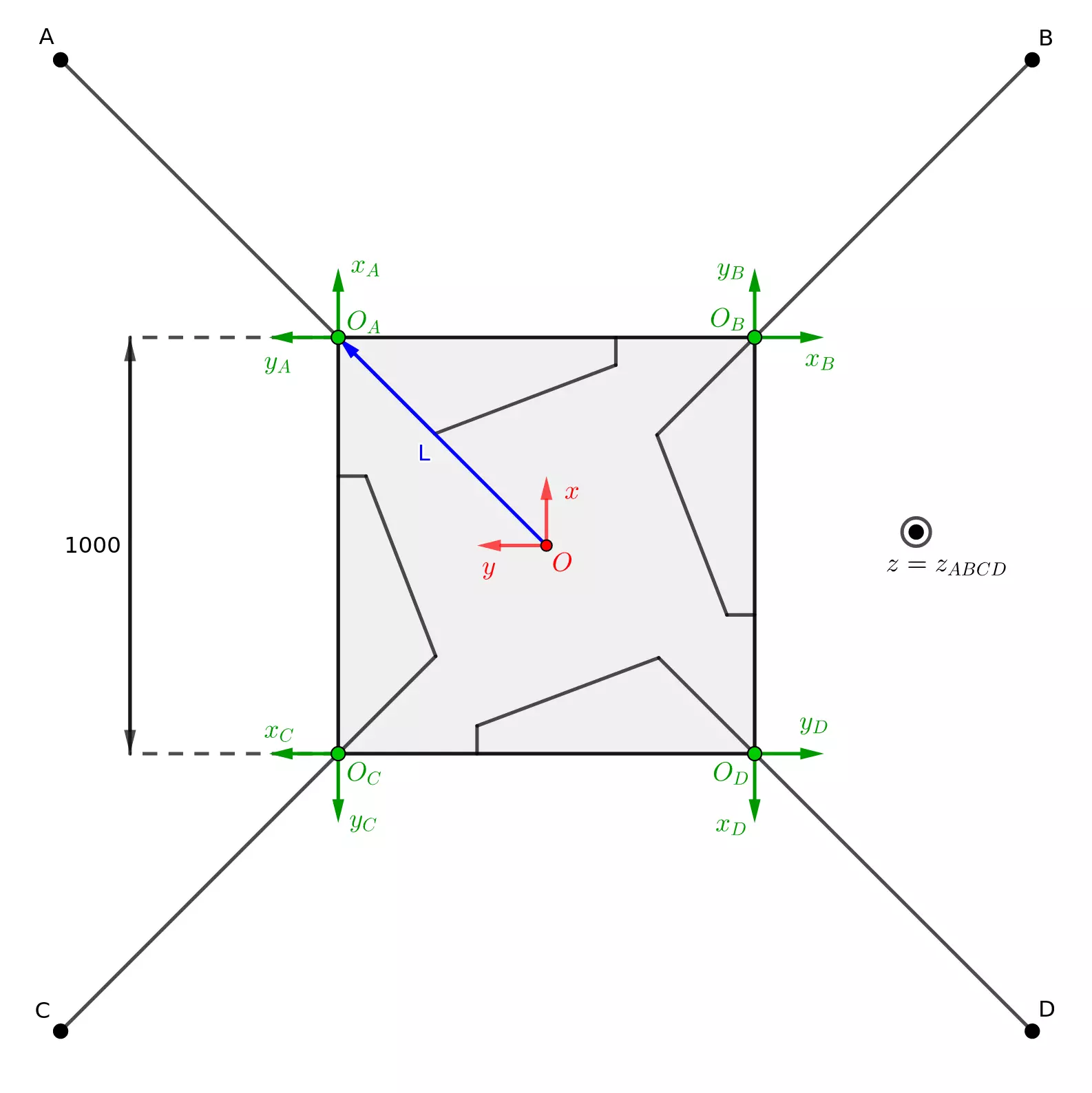
From now on, we will denote \(\Delta V\) as the variations in elongation of the 12 actuators, and \(\Delta X\) as the variations in position of the foot ends in the robot’s reference frame \((\overrightarrow{x}, \overrightarrow{y}, \overrightarrow{z})\). The new transformation matrix between these vectors will be called \(J_{12}\):

We can then observe that using rotation matrices, it is easy to express \(J_{12}\) from \(J_3\) which was computed in the previous section:

The Jacobians \(J_2\), \(J_3\) and \(J_{12}\) computed allow us to develop control algorithms for a single leg in its plane, a leg in its reference frame, and all the legs in the Megabot’s reference frame using a QP solver. Nevertheless, the important issue of managing the center of gravity can also be addressed during the control phase, which is why we will incorporate it into our equations.

Center of Gravity Management

Indeed, an important issue that we aim to solve is maintaining the projection of the robot’s center of gravity inside its support polygon, which is the convex polygon formed by the contact points between the ground and the robot. If the center of gravity of the Megabot were to move outside this area, it would tip over, which would modify its legs on the ground and distort any movement planning.

We have implemented two main control modes, each with its advantages and disadvantages. The first simply constrains the center of gravity to remain above the support polygon by adding constraints in the QP solver. The second allows us to input not only a trajectory for the robot’s legs but also for its center of gravity.

In both cases, it is necessary to develop the Jacobian associated with the displacement of the Megabot’s center of gravity. By knowing the weight of each part of the Megabot, it is possible to determine the variations \(\Delta C\) of the center of gravity from \(\Delta V\) and the Jacobians of the direct kinematic model. In fact, the position of the center of gravity is just a linear combination of the positions of each of the robot’s joints. We thus obtain a relationship of the type:

Center of Gravity Constraint

Once the Jacobian \(J_C\) has been ewpressed, it becomes possible to use the variables \(G\) and \(h\) of the QP solver to constrain the center of gravity. By setting \(G = J_C\) and choosing \(h\) according to the constraints to be applied to the center of gravity, the solver will then ensure that:

Note that here each row of \(G\) and \(h\) corresponds to a constraint on a coordinate of the center of gravity. In practice, we want to constrain the projection of the center of gravity within the support polygon, so \(G\) must be constructed such that each of its rows is a linear combination of the rows of \(J_{C}\), while \(h\) would contain the corresponding constraint values. If we need \(n\) constraints on the coordinates of the center of gravity to keep it within the support polygon, \(G\) and \(h\) would then consists of \(n\) rows.

This solution provides a form of safety while giving the center of gravity some freedom. It seems suitable for a robot with a constant support area during its movement because, in this case, it allows us to constrain the center of gravity to this area and no longer worry about it during the planning phase.

Unfortunately, this is not the case for the Megabot, which is why we opted for the second solution that offers exact control of the center of gravity but, in return, requires its inclusion in the planning phase.

Center of Gravity Control

To control the position of the center of gravity, we need to integrate it into the inputs of the QP solver. We then obtain the following relationship using the previous notations:

The newly constructed Jacobian \(J_{15:12}\) allows us to account for the position of the center of gravity in our forward kinematics. However, the matrix \(J_{15:12}\) cannot be directly used by the QP solver because the matrix \(J_{15:12}\hspace{0.15cm}^TJ_{15:12}\) is singular (see the proof provided at the beginning of the section). One solution to circumvent the singularity of this matrix is to add a regularization term to our minimization.

Details of the addition of a regularization term

Planning

The planning phase involves developing the movement independently of the control-related considerations. It is about knowing what the robot will do and not how it will do it, and this is translated into the implementation of algorithms providing successive positions for the robot’s legs and center of gravity.

Trajectory Development

Our goal was to allow the Megabot to move in a curve. Therefore, we first sought to translate a directional input (2 dimensions) and a rotational input (1 dimension) into a trajectory for the Megabot. This modeling aims to control the robot using a controller with two joysticks.

The direction defines the vector \(\overrightarrow{d}\) represented in the following diagram, while the rotation value defines the position of the center of rotation \(R\) along the axis perpendicular to the direction: the closer the value is to 0, the less pronounced the curve is, and the farther \(R\) is, with positive rotation placing \(R\) to the right and negative rotation placing it to the left. The trajectories of the 4 legs are then determined by tracing the circles centered at \(R\) passing through their ends.

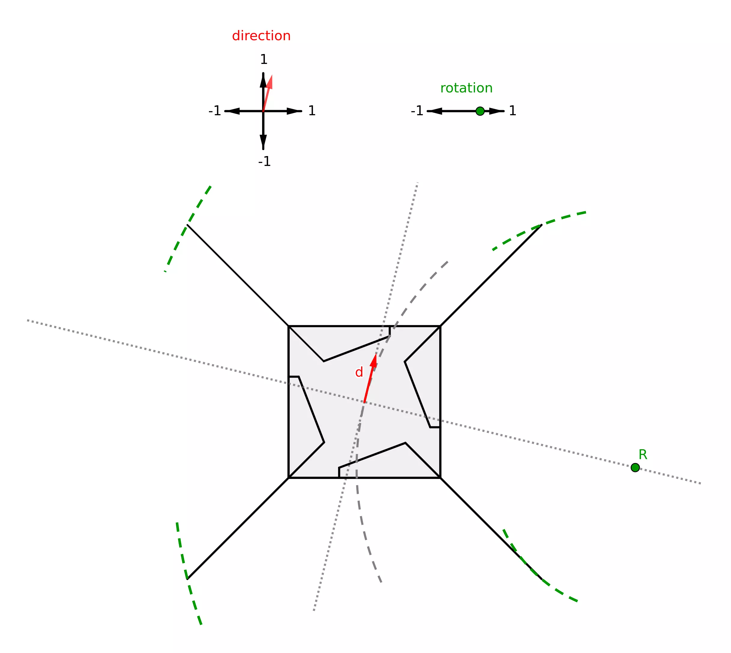
In the case of a zero direction and rotation, \(R\) is placed at the center of the Megabot. In the case of zero rotation and a direction, the trajectories of the legs are simply straight lines parallel to the direction axis.

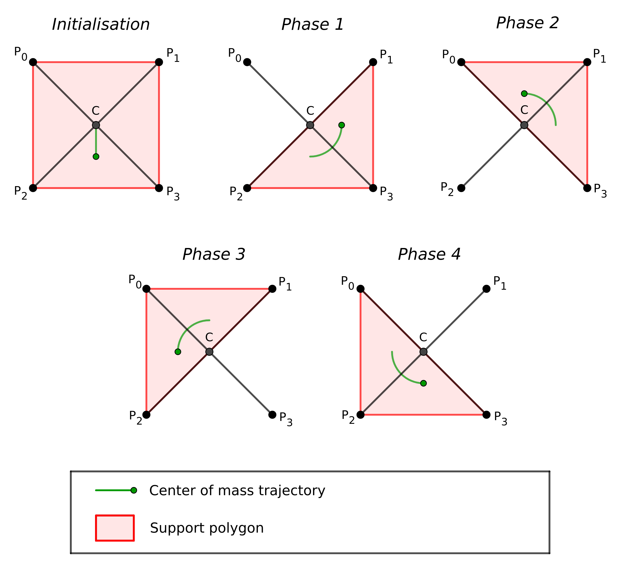
Once the trajectories of the 4 legs were determined, we considered the management of the robot’s center of gravity. The chosen solution to ensure that the center of gravity remains constantly above the support triangle was to have it follow a circular trajectory around the intersection of the diagonals of the polygon formed by the ends of the 4 legs \(P_0\), \(P_1\), \(P_2\) and \(P_3\) during their movement. We will refer to this point as \(C\) in the subsequent explanations. This choice led us to break down the walking motion into 4 phases, preceded by an initialization phase:

Walking Algorithm

Once the trajectories of the 4 leg ends and the center of gravity were established, we discretized the paths of the legs and the center of gravity for each of the phases outlined in the previous figure. The point \(C\) is updated at each step of this discretization, ensuring that the center of gravity remains above the support polygon.

During the initialization phase, the 4 legs are fixed on the ground, and the center of gravity is moved to the rear of the Megabot. Then, during each of the following phases, one leg is lifted, moved along its trajectory, and then lowered while the center of gravity completes a quarter turn around \(C\). This strategy involves moving the legs one by one in a counterclockwise direction. The control algorithm implemented in the Control section translates this command into actuator elongations to perform the walking motion.

Simulation

In order to verify our walking algorithm, it is necessary to perform a simulation of the Megabot. Indeed, although we carried out unit and integration tests of our functions during development, testing the walking directly on the real Megabot would be premature, as if we observed discrepancies between the result and the expected behavior, there would be no guarantee that the error would originate from our algorithmic part and not from our electronics or mechanics.

To simulate the physics during the Megabot’s walking tests, we chose to use PyBullet. This choice required the creation of an URDF file containing a model of the Megabot.

The URDF format represents robots as a tree of parts connected by joints (pivot, slider, etc.). This common modeling approach is suitable for robots with actuated joints, but it prevents the formation of cycles and thus any geometric closure within the robot’s structure. Since all of the Megabot’s movements rely on kinematic loops at the actuator level, it was necessary to find a way to bypass this issue. The solution was to create an incomplete kinematic model and add constraints to close the loops in PyBullet afterwards.

The first step was modeling the Megabot in OnShape, including as many details as possible and specifying the weight and inertial matrices for each part. All the connections between parts were created in an assembly, except for those leading to geometric closures, and the OnShape model was then converted to URDF using the \(\verb|onshape-to-robot|\) tool.

Once the URDF was generated, the geometric closure constraints were built using PyBullet, and the walking simulation was performed.